
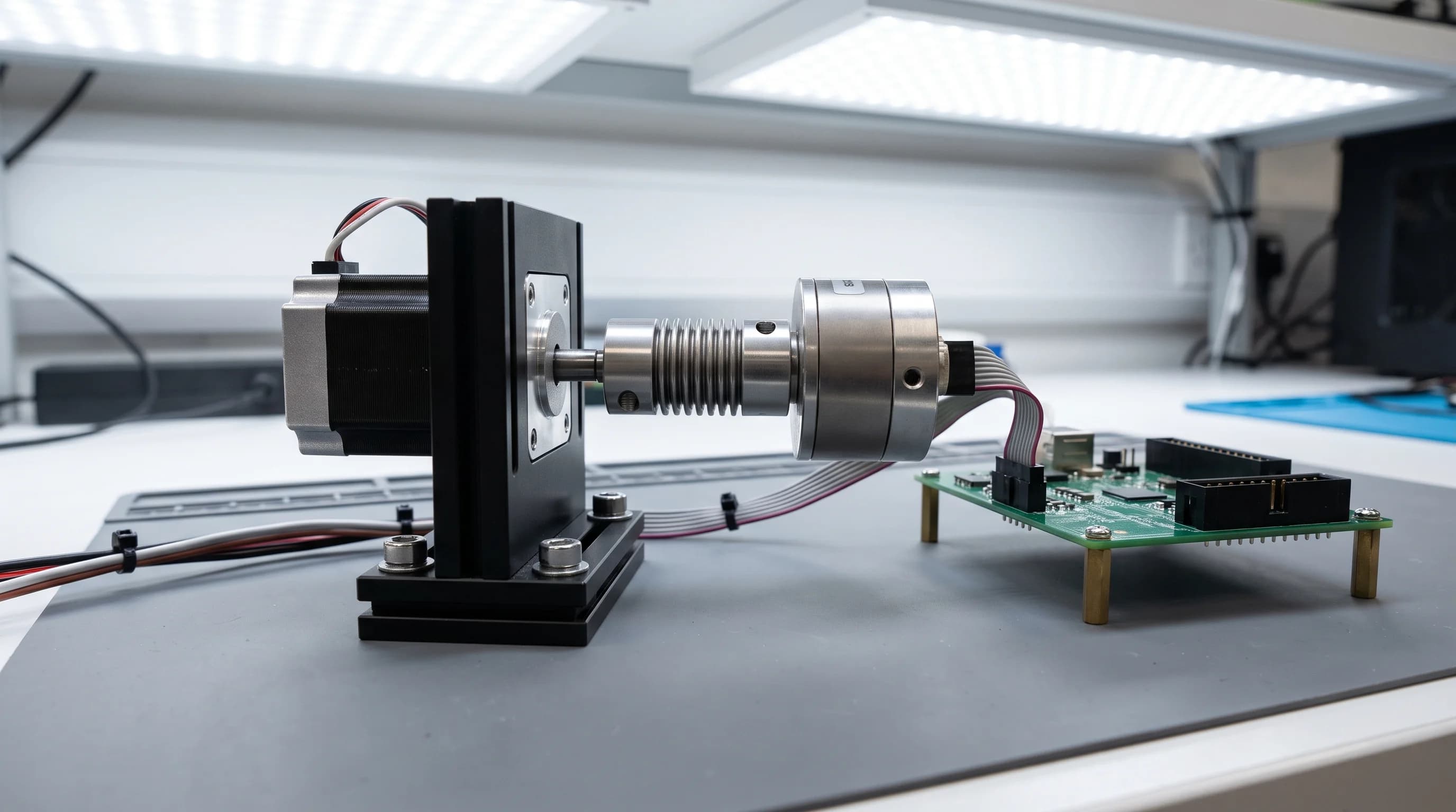
A policy that passes in simulation and fails on the arm has four candidate causes, and each is settled by a different measurement rather than by more randomisation. Contact is three friction numbers in MuJoCo (sliding, torsional and rolling, default 1 0.005 0.0001) plus solref and solimp, and the default condim of 3 leaves the torsional and rolling coefficients unused until you raise it to 4 or 6. Actuator and controller error is fitted, not guessed: a small network trained on under four minutes of logged joint data reached 0.740 Nm average torque error against 3.55 Nm for the zero delay, infinite bandwidth model, 4.8 times better on validation and 5.9 times better on held-out test data. Latency is the cause the simulator never charged you for, and LeRobot's own defaults encode the assumption that one inference fits inside one 33 ms control tick, which is a constant in the codebase and not a measurement of your rig. Randomise only what you could not instrument: the 2017 dynamics randomization work reached 95 randomised parameters and put control timing among them, sampling a 0.04 s base timestep plus an exponential tail averaging 1 to 8 ms. A simulation screen ranks checkpoints rather than predicting a success rate, and on three tasks with six checkpoints the visual matching protocol averaged a Pearson r of 0.924 against 0.308 for ranking by validation MSE. Start this week by timestamping one control loop end to end and comparing the total against your simulator's control timestep.
The ideal actuator model assumes no communication delay and infinite bandwidth: whatever torque you command appears instantly and exactly. Measured against a real quadruped's joints, that assumption carried 3.55 Nm of average torque error, while a small network trained on under four minutes of logged data from the same joints carried 0.740 Nm (arXiv:1901.08652). The sim to real gap is not one phenomenon with one fix. It is a small number of specific, separately measurable errors, and that one is the error you inherit by changing nothing.
This post assumes the boring failures are already excluded. If the policy has never produced sensible motion on hardware, the problem is more likely the dataset-to-policy binding than the physics, and the triage for a 0 percent run settles that in an hour. What the gap is and which task families it hits hardest is covered in our comparison of teleoperation, simulation and human video. What is left is the causal ordering: telling contact error from actuator error from latency error from appearance error, deciding which to identify rather than randomise, and knowing which measurement on the real arm closes each branch.
Ordering matters more than technique, because every one of these has a plausible story attached to it and stories are cheap. A measurement that eliminates a branch is not.
Write down what the simulation number measured
Before the causes, the comparison. A simulated success rate and a hardware success rate are outputs of two different procedures, and unless both are written down they are not comparable. Four things have to match: the initial states, the success predicate, whoever applies that predicate, and the policy checkpoint. Change one and you have measured a different task.
Start with the cheap mismatches. The simulation run samples object poses from a distribution; the hardware run uses the handful of placements a technician can set up reliably. The simulation predicate is a threshold on ground truth state; the hardware predicate is a person deciding whether the part went in. Both numbers can be correct and not comparable.
So fix the comparison design first, and change exactly one variable per run. How many rollouts it takes before a difference between two numbers means anything is a separate question, worked out in how many trials it takes to evaluate a robot policy. Do not size it by intuition.
Four causes, one symptom, and the measurement that settles each
"The policy fails on hardware" is a single symptom with four causes underneath it. Each one has a signature in when the episode breaks, and each one has a measurement that either implicates it or removes it from the list.
Work them in that order, on cost per branch eliminated rather than likelihood. Latency is first because it needs a stopwatch and no hardware change, and because a loop that overruns its tick corrupts every measurement taken afterwards. Contact is second because one afternoon of bench work settles it. Actuator dynamics are third because the fit is real work. Appearance is last because it announces itself: a rollout where the arm reaches the right place and fails at contact has already eliminated that branch, and what to do when it has not is a camera placement problem.
Nobody publishes a breakdown of how often each branch is at fault, so any percentage split you are shown has no primary source behind it. Plan around the elimination order instead.
| Branch | Signature on hardware | The measurement that settles it | What the fix costs |
|---|---|---|---|
| Control-loop latency | Pauses and jerk at chunk boundaries; degrades as the policy gets bigger; worse on the fast segments | Timestamp one loop end to end: exposure, transport, preprocessing, inference, network hop, command. Compare the total to the simulator's control timestep | Hours. A serving change, or a retrain with randomised timing |
| Contact and friction | Failure lands at the instant of contact: slip, rotation in the fingers, binding on insertion | On the bench, measure a slip angle or a push-to-move force for the real pair, then reproduce the same push in the simulator | A day of bench work plus a parameter sweep |
| Actuator and controller dynamics | Trajectory shape is right, timing is wrong: lag, overshoot, ringing on fast segments | Replay a logged open-loop action sequence through the simulator and compare the resulting end-effector pose trajectory against the logged real one | Days. A fit, and possibly a model change |
| Appearance and viewpoint | Failure lands before contact: the arm reaches to the wrong place, or does not commit at all | Freeze the scene and change one visual variable at a time; check the camera extrinsics against the rig that recorded the data | Cheap if the rig is intact, expensive if it moved |
Contact and friction: identify one pair, do not sweep the defaults
Contact is where a simulator is least like a bench, and MuJoCo is honest about which numbers are in play. In the XML reference at 3.13.0 the geom friction attribute holds three coefficients, defaulting to 1 0.005 0.0001: sliding friction along both axes of the tangent plane, torsional friction around the contact normal, and rolling friction around both tangent axes. Softness lives in two more, whose numeric defaults sit in the modeling chapter rather than in the XML reference, which only points at the solver section: solref, default 0.02 1, the time constant and damping ratio of the virtual spring damper used for constraint stabilisation, and solimp, default 0.9 0.95 0.001 0.5 2, which parameterises how impedance varies with the constraint violation.
A fourth attribute decides whether two of those coefficients do anything at all. condim defaults to 3, documented as a regular frictional contact that opposes slip in the tangent plane. Torsional friction, the torque opposing rotation around the contact normal, requires condim="4". Rolling friction requires condim="6". A gripper that lets the part spin between the fingertips in reality but holds it in simulation is a condim question before it is a friction-coefficient question, because at the default the torsional coefficient you were tuning is inert. The computation chapter calls condim="4" useful for modelling soft fingers and notes it can substantially improve the stability of simulated grasping.
Get the measurement before the sweep. The sliding coefficient is the tangent of the angle at which a flat object begins to slip under gravity, which is a protractor and a plate. Torsional and rolling coefficients have units of length in MuJoCo, read as the diameter of the contact patch and the depth of local deformation, so a caliper on the fingertip pad beats a blind sweep.
Then change the pair, not the world. A contact/pair element declares a named geom pair whose properties replace those of the individual geoms, which keeps the identification local to the two surfaces that decide the task.
<mujoco>
  <!-- the documented baseline you are departing from, shown so the diff is visible -->
  <option timestep="0.002" integrator="Euler" cone="pyramidal"/>

  <default>
    <geom friction="1 0.005 0.0001"
          solref="0.02 1"
          solimp="0.9 0.95 0.001 0.5 2"/>
  </default>

  <!-- geom1 and geom2 name geoms in your own worldbody.
       condim=4 makes the torsional coefficient live; at the default 3 it is unused.
       pair friction is 5 numbers: tangential, tangential, torsional, rolling, rolling.
       These values are an example to sweep, not a recommendation. -->
  <contact>
    <pair geom1="fingertip_pad" geom2="workpiece"
          condim="4"
          friction="0.6 0.6 0.01 0.0001 0.0001"
          solref="0.02 1"
          solimp="0.9 0.95 0.001 0.5 2"/>
  </contact>
</mujoco>
Two rules on the sweep. Move one coefficient per run, because the solver couples them and a two-parameter sweep gives you a surface you cannot read. And re-run the same logged push each time, scoring the simulated trajectory against the real one, rather than re-running the policy, which mixes the parameter change with the policy's own variance. Which engine you run this in is a decision of its own.
Actuator and controller dynamics are measured, not randomised
The default actuator is a fiction with a known cost. The 2019 quadruped work states it plainly: the ideal actuator model assumes no communication delay and an actuator that generates any commanded torque instantly. Measured against real series-elastic actuators it carried 3.55 Nm of average torque error on validation data and 5.74 Nm on data collected under the trained locomotion policies. A small network fitted to logged joint data carried 0.740 Nm and 0.966 Nm on the same two sets: 4.8 times better on validation, 5.9 times better on the held-out test data.
The identification recipe is the transferable part, and it is cheap. A parameterised controller drove the feet along sine wave trajectories, with amplitude varied from 5 to 10 cm and frequency from 1 to 25 Hz, and the robot was disturbed by hand during collection. Joint position errors, joint velocities and torques were logged at 400 Hz across 12 identical actuators, putting collection under four minutes and producing over a million samples. Roughly 90 percent trained the model and the rest validated it. The model is small: three hidden layers of 32 units. The paper is explicit that excitation must cover a wide frequency spectrum, because narrow excitation produced a model that oscillated unnaturally even during training.
The reason to fit rather than derive is stated in the same work: these actuators involve nonlinear and nonsmooth dissipation, cascaded feedback loops and internal states that are not directly observable, and a parametric model of them runs to nearly a hundred estimated parameters.
That result describes series-elastic actuators. A low cost position controlled arm with a simple servo loop may be adequately described by a fixed delay plus a first order lag, which is two parameters and an afternoon. Start there and escalate only when the residual says the simple model is not enough.
For the controller rather than the actuator there is a cheaper published procedure that needs no new data collection. Take an action sequence logged on the real robot, unroll it open-loop in the simulator from the same starting pose, and score the simulated 6D end-effector pose trajectory against the recorded one. The 2024 simulated-evaluation work defines that loss as mean translation error plus mean rotation error and fits the controller's stiffness and damping against it with simulated annealing over a normalised search range (arXiv:2405.05941), using a handful of trajectories from a demonstration dataset you already have. This is a trajectory match run inside the simulator, not a hardware replay, and it says nothing about your recording pipeline. Whether the replayed actions are joint targets or end-effector deltas changes what the fit means, which is the action space argument.
The simulator never charged you for inference time
A simulator advances by a control timestep and then asks the policy for an action. It never notices how long the answer took to arrive. On hardware that delay sits inside the loop, and the policy acts on a view of the world that is one or two ticks stale.
The tooling encodes the optimistic assumption as a default. In LeRobot v0.6.1, async_inference/constants.py sets DEFAULT_FPS = 30 and DEFAULT_INFERENCE_LATENCY = 1 / DEFAULT_FPS: one inference is expected to fit inside one 33 ms control tick. Whether it does is a property of your policy and your card. LeRobot's documentation puts a pi0-class policy at 14 GB of memory at inference time against roughly 2 GB for SmolVLA, and the documented consequence of synchronous execution is idle frames, where the robot waits for the next action chunk. On the bench that reads as a stutter at chunk boundaries, worse the larger the policy.
Measure it rather than model it. End-to-end latency is the sum of camera exposure and transport, preprocessing, inference, the network hop if the policy server is not on the robot's host, and actuator command latency. Log the deltas, sum them, and compare against the control timestep you simulated with. The async serving path reads out the failure mode directly, because the client can plot its own action queue.
pip install 'lerobot[async]'

# terminal 1: policy server, timings stated rather than inherited
python -m lerobot.async_inference.policy_server \
    --host=127.0.0.1 \
    --port=8080 \
    --fps=30 \
    --inference_latency=0.033 \
    --obs_queue_timeout=1

# terminal 2: client, with the action queue plotted so starvation is visible
# --robot.type, --robot.id and --robot.port are rig specific.
# --robot.cameras is left out here: its keys have to match the ones the policy expects.
python -m lerobot.async_inference.robot_client \
    --robot.type=so100_follower \
    --robot.id=<your robot id> \
    --robot.port=<your serial device> \
    --task="<the task string you recorded with>" \
    --server_address=127.0.0.1:8080 \
    --policy_type=smolvla \
    --pretrained_name_or_path=lerobot/smolvla_base \
    --policy_device=cuda \
    --actions_per_chunk=50 \
    --chunk_size_threshold=0.5 \
    --aggregate_fn_name=weighted_average \
    --debug_visualize_queue_size=True
A queue that trends toward empty is the measurement. The documentation's instruction is to reduce fps when you consistently run out of actions in queue, which is an admission that inference time sets your control rate. One number to read carefully: chunk_size_threshold defaults to 0.5 in the v0.6.1 source while the tutorial table lists 0.7, and actions_per_chunk has no default in the source because the field is required. Pass both explicitly. The 0.5 above is the source value; the 50 is the documentation's example, chosen rather than inherited, because there is no source default to inherit. What those two levers trade off is worked through in our VLA comparison.
If the measurement says latency is your branch, there are two fixes with different bills. Retrain with randomised action timing, which is the next section. Or change the serving path: real time chunking generates the next action chunk while the current one executes, freezing the actions guaranteed to execute and inpainting the rest, and it applies to any diffusion or flow based VLA with no retraining (arXiv:2506.07339). In LeRobot that is the rtc inference backend, against the default sync backend that makes one policy call per control tick. We found no head-to-head between the two on a common task, so treat them as branches with different costs rather than a ranked pair.
Randomise only what you could not instrument
Domain randomization did not start as a physics technique. In the 2017 paper that explored it, what varied was rendering, and its reported result is an object detector accurate to 1.5 cm, trained only on simulated images with non-realistic random textures (arXiv:1703.06907). That is a perception claim about localisation. Neither that paper nor the dynamics paper below states that randomisation closes the gap on contact-rich manipulation, so do not carry that claim into a design review.
The dynamics version is the one that matters here, and its parameter table is the concrete answer to what randomising dynamics actually means (arXiv:1710.06537).
Eight groups, plus Gaussian observation noise applied per step, adding up to 95 randomised parameters in that setup. Mass, damping, friction, gains and timing. No textures.
The last row is the one to steal. The timestep between actions is how long an action is applied before the policy is queried again, and the paper describes it as a simple model of the latency exhibited by the physical controller. It is sampled as a 0.04 s default control timestep plus an exponential draw whose rate parameter ranges from 125 to 1000 per second, a mean added delay of 1 to 8 ms. The rate parameter is fixed within an episode and the delay is redrawn every step, so the policy trains against jitter rather than a constant lag. Control latency sits inside the randomisation set, next to link mass: a modelled quantity, not an excuse reached for after the hardware run disappoints.
So the rule is narrow. Identify what you can instrument: the friction of your pair, the delay and lag of your servo, the stiffness and damping of your controller. Randomise what you cannot: unit-to-unit variation across arms, a workpiece mass that changes between batches, and end-to-end latency, which is genuinely distributional because it depends on thermal state, on what else is on the GPU, and on the network. In Isaac Lab, randomisation is a scheduled event term rather than a boolean: an EventTermCfg carries a func and a mode, with interval reserved as a special mode handled by the manager and interval_range_s giving the sampling window. Read the event functions at the tag you have pinned rather than from an article.
And stop. The stopping rule comes from the actuator fit: the learned model landed at 0.740 Nm against a torque sensor resolving 0.2 Nm, close enough to the instrument that more fitting buys nothing verifiable. When the difference between the simulated trajectory and the logged one is within the noise of the instrument that logged it, the model is done, and widening a range past that point costs policy performance for robustness you cannot demonstrate.
| Randomised parameter | Range |
|---|---|
| Link mass | 0.25 to 4 times the default mass of each link |
| Joint damping | 0.2 to 20 times the default damping of each joint |
| Puck mass | 0.1 to 0.4 kg |
| Puck friction | 0.1 to 5 |
| Puck damping | 0.01 to 0.2 N.s/m |
| Table height | 0.73 to 0.77 m |
| Controller gains | 0.5 to 2 times the default gains |
| Action timestep, rate parameter | 125 to 1000 per second |
The screen ranks checkpoints, and it runs inside your perimeter
A simulated evaluation is a screen, not a forecast. The 2024 work that built simulated environments for evaluating real manipulation policies measured this directly, ranking six open-source checkpoints on three Google Robot tasks and reporting rank fidelity rather than success-rate agreement.
Those six rows are two metrics across three evaluation protocols, measured on three tasks with six checkpoints. They are not a general coefficient for sim to real, and the paper's own abstract reports a strong correlation with no number attached to it. The row that earns its place is the first: ranking the same checkpoints by validation loss averaged 0.308, so an offline loss curve orders checkpoints badly and a simulated rollout orders them well. Neither tells you the number the plant will see.
Running the screen is a two-part install, and the first part is a trap. LeRobot's evaluation extra resolves to av and nothing else, so it brings no simulator with it; the environment package is a separate extra named alongside it.
pip install 'lerobot[evaluation,pusht]'

lerobot-eval \
    --policy.path=outputs/train/diffusion_pusht/checkpoints/005000/pretrained_model \
    --env.type=pusht \
    --eval.batch_size=10 \
    --eval.n_episodes=10 \
    --policy.use_amp=false \
    --policy.device=cuda
Where a private deployment changes the answer is in where the environment came from. A screen you re-run across checkpoints has to be reproducible, which means pinning the environment the way you pin the policy. LeRobot can load one from the Hub, and doing so imports and executes Python from a third-party repository inside your process. The consent flag is explicit and the documentation recommends pinning to a commit hash for reproducibility and security; in a plant network neither is advice.
from lerobot.envs import make_env

# lerobot/cartpole-env is the documentation's example repo and a1b2c3d4 stands in
# for a full commit hash. Pin the commit, never a branch, and inside a plant
# network swap the repo id for an internal mirror you control.
envs_dict = make_env("lerobot/cartpole-env@a1b2c3d4", n_envs=4, trust_remote_code=True)

suite_name = next(iter(envs_dict))
env = envs_dict[suite_name][0]
obs, info = env.reset()
The identification data is the part that never leaves. Torque and joint logs from the line, trajectories over your own parts, fixture geometry and bench slip measurements are process data, and they are what turns a generic simulator into a model of your cell. Fitting happens where the data already is.
One deployment detail deserves a look before the policy server moves off the robot's host. It binds an insecure gRPC port and defaults to localhost. Moving it to a shared GPU box does two things at once: it exposes an unauthenticated endpoint that speaks to a moving arm, and it inserts a network hop into the loop you just measured. Segment the link, then re-measure, because the latency you validated was measured without that hop. The wider view of this stack inside a regulated perimeter sits on the physical AI pillar.
| Protocol and metric | Pick Coke Can | Move Near | Drawer | Average |
|---|---|---|---|---|
| Validation MSE, Pearson r (higher better) | 0.464 | 0.230 | 0.231 | 0.308 |
| Variant aggregation, Pearson r | 0.960 | 0.887 | 0.486 | 0.778 |
| Visual matching, Pearson r | 0.976 | 0.855 | 0.942 | 0.924 |
| Validation MSE, MMRV (lower better) | 0.412 | 0.408 | 0.306 | 0.375 |
| Variant aggregation, MMRV | 0.084 | 0.111 | 0.235 | 0.143 |
| Visual matching, MMRV | 0.031 | 0.111 | 0.027 | 0.056 |
The order to work through, and when to stop
Take the four branches in cost order and do not skip ahead on a hunch.
condim before you conclude a coefficient is wrong.Then stop when the residual falls below your measurement noise. A simulator that matches your logs to within the resolution of the instrument that produced them is finished, whatever the success rate still says.
This week, do the cheapest of the four. Put a timestamp at each stage of one control loop, run twenty episodes, and write down the p50 and p95 of the total. Compare that against the control timestep in your simulation config. If the p95 is larger, you have found a cause without touching the physics.
FAQ
Quick answers to the questions this post tends to raise.